Quick Guide#
Here is a quick guide of the template construction using BYOST.
This notebook contains the following sections:
Input data
Construct the buildingblock
Get template from buildingblock
Visualization
Distribution of data
PCA results
GPR results
Template
Template compare with sample
import BYOST
import pandas as pd
import numpy as np
import matplotlib.pyplot as plt
Input data#
You need a data file (the data contains features and measurements) and a condition file (the conditions that you wish the data to be modeled upon).
The input data file need to be a pandas dataframe that has features as columns (e.g., wavelength) and measurements as rows (e.g., flux of each spectrum at those wavelength)
The condition file need to be a pandas dataframe that has 2 conditions (e.g, epoch and sBV) as columns and the corresonding condition of the measurements (matching by index).
# df_data       = pd.read_csv(<your_file_path>)
# df_conditions = pd.read_csv(<your_file_path>)

display(df_data)
display(df_conditions)
| 9342.0 | 9343.0 | 9345.0 | 9347.0 | 9348.0 | 9350.0 | 9352.0 | 9353.0 | 9355.0 | 9357.0 | ... | 11045.0 | 11047.0 | 11050.0 | 11053.0 | 11056.0 | 11059.0 | 11062.0 | 11065.0 | 11068.0 | 11071.0 | |
|---|---|---|---|---|---|---|---|---|---|---|---|---|---|---|---|---|---|---|---|---|---|
| 0 | 0.001144 | 0.001142 | 0.001141 | 0.001140 | 0.001138 | 0.001136 | 0.001135 | 0.001133 | 0.001130 | 0.001128 | ... | 0.000351 | 0.000351 | 0.000350 | 0.000350 | 0.000350 | 0.000350 | 0.000350 | 0.000351 | 0.000352 | 0.000352 |
| 1 | 0.001217 | 0.001213 | 0.001209 | 0.001205 | 0.001200 | 0.001196 | 0.001192 | 0.001188 | 0.001184 | 0.001180 | ... | 0.000399 | 0.000396 | 0.000393 | 0.000390 | 0.000385 | 0.000381 | 0.000376 | 0.000370 | 0.000365 | 0.000360 |
| 2 | 0.001255 | 0.001254 | 0.001253 | 0.001253 | 0.001252 | 0.001251 | 0.001250 | 0.001249 | 0.001248 | 0.001247 | ... | 0.000240 | 0.000239 | 0.000238 | 0.000237 | 0.000236 | 0.000235 | 0.000234 | 0.000234 | 0.000234 | 0.000233 |
| 3 | 0.000975 | 0.000974 | 0.000972 | 0.000970 | 0.000968 | 0.000966 | 0.000964 | 0.000962 | 0.000960 | 0.000958 | ... | 0.000283 | 0.000282 | 0.000281 | 0.000279 | 0.000278 | 0.000276 | 0.000275 | 0.000273 | 0.000272 | 0.000270 |
| 4 | 0.000586 | 0.000585 | 0.000585 | 0.000585 | 0.000585 | 0.000585 | 0.000585 | 0.000584 | 0.000584 | 0.000584 | ... | 0.000351 | 0.000350 | 0.000348 | 0.000346 | 0.000344 | 0.000341 | 0.000339 | 0.000337 | 0.000335 | 0.000333 |
| ... | ... | ... | ... | ... | ... | ... | ... | ... | ... | ... | ... | ... | ... | ... | ... | ... | ... | ... | ... | ... | ... |
| 326 | 0.000957 | 0.000956 | 0.000955 | 0.000955 | 0.000955 | 0.000954 | 0.000954 | 0.000954 | 0.000954 | 0.000955 | ... | 0.000202 | 0.000201 | 0.000201 | 0.000200 | 0.000199 | 0.000198 | 0.000198 | 0.000197 | 0.000197 | 0.000196 |
| 327 | 0.001117 | 0.001117 | 0.001117 | 0.001117 | 0.001117 | 0.001117 | 0.001116 | 0.001116 | 0.001116 | 0.001116 | ... | 0.000423 | 0.000422 | 0.000422 | 0.000422 | 0.000421 | 0.000421 | 0.000421 | 0.000420 | 0.000420 | 0.000419 |
| 328 | 0.001184 | 0.001183 | 0.001181 | 0.001180 | 0.001179 | 0.001177 | 0.001176 | 0.001174 | 0.001173 | 0.001172 | ... | 0.000322 | 0.000322 | 0.000321 | 0.000321 | 0.000320 | 0.000320 | 0.000319 | 0.000319 | 0.000318 | 0.000318 |
| 329 | 0.001105 | 0.001104 | 0.001103 | 0.001102 | 0.001101 | 0.001100 | 0.001100 | 0.001099 | 0.001098 | 0.001098 | ... | 0.000268 | 0.000267 | 0.000267 | 0.000266 | 0.000265 | 0.000265 | 0.000264 | 0.000263 | 0.000262 | 0.000262 |
| 330 | 0.001009 | 0.001009 | 0.001009 | 0.001010 | 0.001010 | 0.001011 | 0.001012 | 0.001013 | 0.001014 | 0.001015 | ... | 0.000154 | 0.000153 | 0.000152 | 0.000152 | 0.000151 | 0.000150 | 0.000149 | 0.000149 | 0.000148 | 0.000148 |
331 rows × 766 columns
| epoch | sBV | |
|---|---|---|
| 0 | 3.608522 | 1.013 |
| 1 | 10.414827 | 1.013 |
| 2 | 17.162779 | 1.013 |
| 3 | 22.024722 | 1.013 |
| 4 | 32.667662 | 1.013 |
| ... | ... | ... |
| 326 | 67.777483 | 0.884 |
| 327 | 1.679203 | 0.692 |
| 328 | 6.589792 | 0.692 |
| 329 | 11.498910 | 0.692 |
| 330 | 61.289914 | 0.692 |
331 rows × 2 columns
Construct the buildingblock#
BYOST.build.make_buildingblock(df_data,df_conditions,
                              normalize_method='intergrated_flux', normalize_wave_range=None,standardize_std = False,
                              n_components=10,
                              length_scales=[10.0,0.1],remove_outliars = True,n_restarts_optimizer=20)
Required Input:
df_data: pandas dataframe of the spectra on the common wavelenght grid, with wave as column namesdf_conditions: pandas dataframe of the conditions corresponding to df_data, e.g., epochs and sBVs
Optional arguements that could be used to prepare the data
normalize_method: default = ‘intergrated_flux; or None, “mean_flux” or “intergrated_flux” - None: take the input data as it is - “mean_flux”: normalize by dividing the mean flux in the selected range - “intergrated_flux”: normalize by dividing the intergrated flux in the selected rangenormalize_wave_range: default = None, which is normalized on the given data, or 2-element list ([lambda_left,lambda_right])standardize_std: default = False, if=True, standardize the input data by standard deviation of each column
Optional arguements for the PCA step
n_components: default = 10, the number of the components you would like to keep for furhure analysis
Optional arguements for the GPR step
length_scales: default [10, 0.1], the length scale of the RBF kernal for condition_1 and condition_2 The GPR depends on these initial scale values, try out the optiminal length scale for your data set!! (this is a little bit similar to the smoothness of the GP preditons, larger scale will return smoother precition, smaller scale will have more details)remove_outliars: default = True, ignore the local PC ourliars that are beyond 5sigma*global_stdn_restarts_optimizer: number of restart of the optimizer
Output: df_buildingblocks: pandas dataframe contains resulting PCA and GPR
## to build a building block (contains fitted PCA and GP) given data and conditions

## sometimes warning of Guassian Process parameters did not converge
import warnings
warnings.filterwarnings("ignore")

df_buildingblock = BYOST.build.make_buildingblock(df_data,df_conditions,normalize_method='intergrated_flux',n_components=10)
If you have dataset from different wavelength region, you can build them seperately and then concat them, make sure the regions are overlapped, e.g.:
df_buildingblock2 = BYOST.build.make_buildingblocks(df_data2,df_conditions2,n_components=2)
df_buildingblocks = pd.concat([df_buildingblock,df_buildingblock2],axis=0,ignore_index=True)
To save the df_buildingblock to pickle file for storage the fitted pca and gp, pickle file is recommended
df_buildingblocks.to_pickle('df_buildingblocks.pkl')
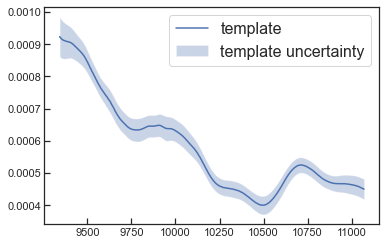
##Get template from buildingblock
BYOST.template.get_template(df_buildingblock,condition1,condition2,
                            PC_select_method = ['GPR_score_threshold',0.2],
                            return_template_error=False,
                            error_MC_num = 1000,return_MC_spectra=False)
Required Inputs:
df_buildingblock: pandas dataframe contains resulting PCA and GPR if there is more than 1 wavelength region (df_buildingblock.shape[0]>1), the wavelength must be aranged from blue to red in the dataframe, and has overlap in neighbouring region in order to enable mergingcondition1: scaler (this parameter corresponding to the first columns of the given df_conditions for buildingblock)condition2: scaler (this parameter corresponding to the second columns of the given df_conditions for buildingblock)
Optional arguements:
PC_select_method: default [‘GPR_score_threshold’,0.2], method of selecting which PCs to keep for template flux constructionGPR_score_threshold: keep PCs that has GPR R^2 >= GPR_score_thresholdPCA_variance_pctg_threshold: keep PCs up to the one that has total_variance >= PCA_variance_pctg_threshold, eg, [‘PCA_variance_pctg_threshold’,94] as >=94%fixed_PC_number: keep n (n=fixed_PC_number) first PCs, eg. [‘fixed_PC_number’,6] as keeping first 6 PCs
return_template_error: default False; If True, return the template flux errorerror_MC_num: will be used is return_template_error=True, the number of the interations to get the template flux error.return_MC_spectra: default False, if True, return all the possible spectra during the MC.
Output: tuple
tuple: template_wavelength, template_flux (if
return_template_error=False)tuple: template_wavelength, template_flux, template_error (if
return_template_error=Trueandreturn_MC_spectra=False)tuple: template_wavelength, template_flux, template_error, MC_template_flux (if
return_template_error=Trueandreturn_MC_spectra=True)
cond1 = -10.  # in example, cond1 is epoch of the spectrum
cond2 = 0.65  # in example, cond2 is sBV of the SN

wave,flux,flux_err = BYOST.template.get_template(df_buildingblock,cond1,cond2,return_template_error=True)

plt.plot(wave,flux,label='template')
plt.fill_between(wave,flux-flux_err,flux+flux_err,alpha=0.3,label='template uncertainty')
plt.legend(fontsize=16)
<matplotlib.legend.Legend at 0x7fcd94024eb0>
Visualization#
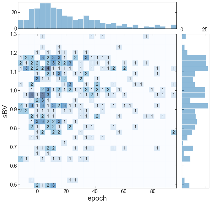
Distritbuion of data#
The 2 distribution of the data in the given conditions
fig = BYOST.visualize.hist_2d(df_conditions)
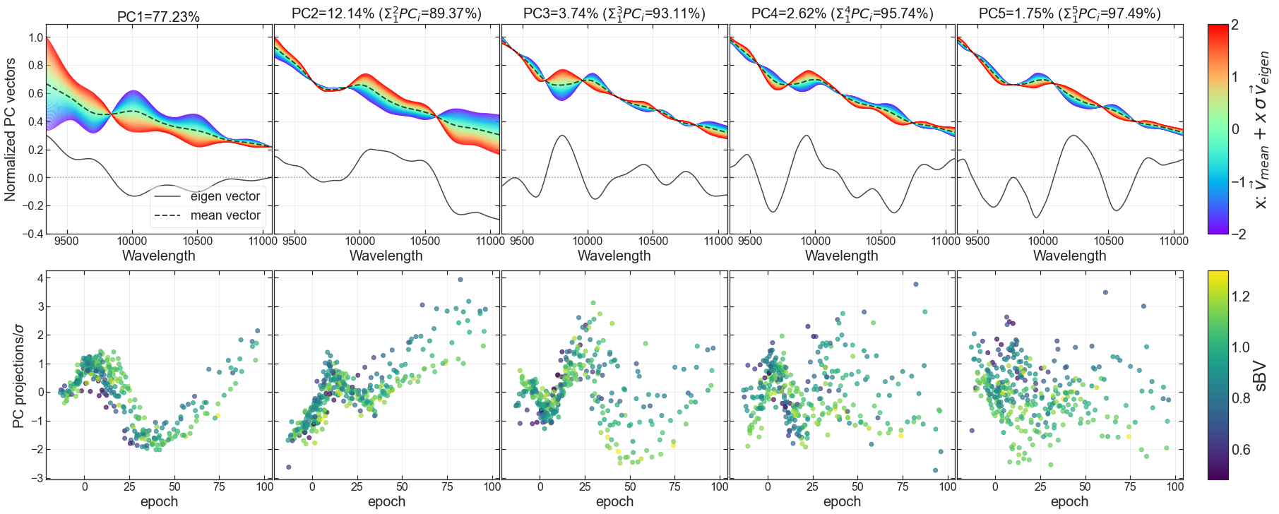
PCA results#
BYOST.visualize.plot_PCA(df_buildingblock,df_conditions,n_components=None,PC_vector_sigma=1)
Required Input:
df_buildingblock: pandas dataframe contains resulting PCA and GPRdf_conditions: pandas dataframe of the conditions corresponding to df_spectra, e.g., epochs and sBVs
Optional Inputs:
n_components: number of PCs to plot, default None and will plot all produced PCsPC_vector_sigma: default 2, the PC projection sigma when plotting the variance represented by the PC vectors
Output: Fig of PCA results:
first row is PC vectors and its variation,
second row is PC projections vs given conditions
fig = BYOST.visualize.plot_PCA(df_buildingblock,df_conditions,n_components=5,PC_vector_sigma=2)
GPR results#
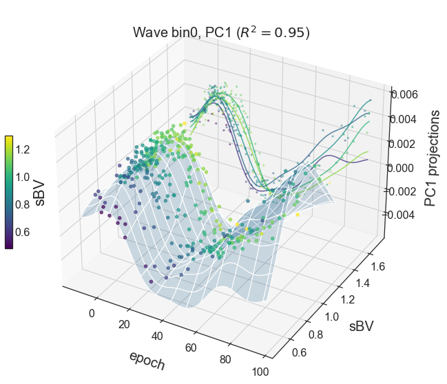
BYOST.visualize.plot_GPR(df_buildingblock,df_conditions,Wave_bin_ID=0,PC='PC1',view_angle = [32,300])
Inputs:
df_buildingblock: pandas dataframe contains resulting PCA and GPRdf_conditions: pandas dataframe of the conditions corresponding to df_spectra, e.g., epochs and sBVsWave_bin_ID: default 0, the row index of the df_buildingblockPC: default ‘PC1’view_angle: default [32,300],the viewing angle of the 3D plot
Output: Fig of GPR results, a 3D illustration of the GP fits and the 2D projections on the back
fig = BYOST.visualize.plot_GPR(df_buildingblock,df_conditions,PC='PC1')
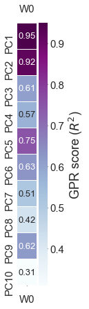
## plot GPR scores (R^2)

fig = BYOST.visualize.plot_GPR_score(df_buildingblock)
Template#
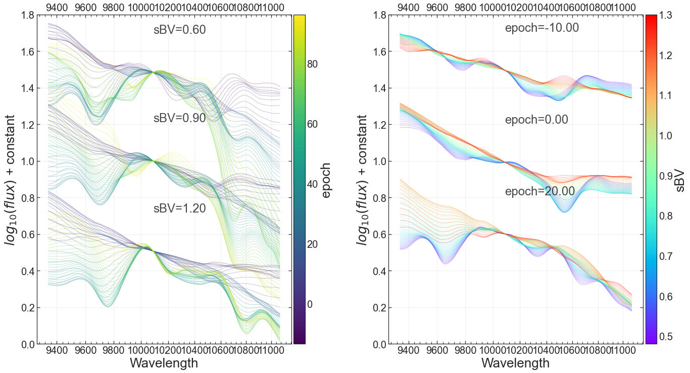
BYOST.visualize.plot_template(df_buildingblock,df_conditions,
                              matching_wave_position=None,y_offset_gap=1.0,
                              condition1_sample=None,condition2_sample=None,
                              condition1_colormap = 'rainbow',condition2_colormap = 'viridis',
                              log_x=True, log_y=True)
Input:
df_buildingblock: pandas dataframe contains resulting PCA and GPRdf_conditions: pandas dataframe of the conditions corresponding to df_spectra, e.g., epochs and sBVsmatching_wave_position: default will match the flux at the median wavelength postiony_offset_gap: the offset in yaxis between the sampling template, default 1.0condition1_sample: default will sample the mean-std, mean, mean+std of the condition1 values while varying condition2condition2_sample: default will sample the mean-std, mean, mean+std of the condition2 values while varying condition1condition1_colormap: the color secheme for varying condition1, default rainbowcondition2_colormap: the color secheme for varying condition1, default viridislog_x: default True, wavelength is plotted in log scalelog_y: default True, flux is plotted in log scale
Output:
Fig of template variation, with 2 panels:
left panel: variation within condition1 while keeping condition2 fixed at certain values
right panel: variation within condition2 while keeping condition1 fixed at certain values
fig = BYOST.visualize.plot_template(df_buildingblock,df_conditions,
                                    y_offset_gap = 0.5,
                                    condition1_sample=[-10,0,20],condition2_sample=[0.6,0.9,1.2],
                                    condition1_colormap = 'viridis',condition2_colormap = 'rainbow')
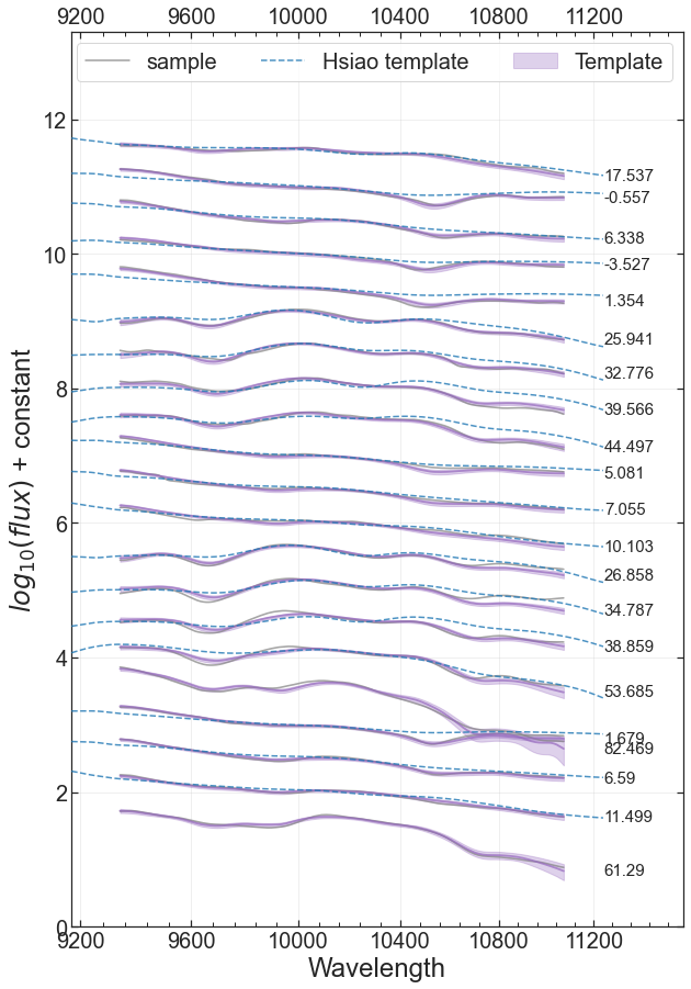
Template compare with sample#
BYOST.visualize.comp_template_with_sample(df_buildingblock,df_sample_with_conditions,\
                              label_cols = ['cond1','cond2'],legend_label='sample',\
                              co_comp_Hsiao_temp = False,\
                              log_x=True,log_y=True,fig_ax=None,\
                              plot_gap = 0.7, ymax_shift = 0):
Input:
df_buildingblock: pandas dataframe contains resulting PCA and GPRdf_sample_with_conditions: pandas dataframe contains [‘wave’,’flux’,’cond1’,’cond2’] in columnslabel_cols: default [‘cond1’,’cond2’], the lables shows at the end of the each spectrumlegend_label: default ‘sample’co_comp_Hsiao_temp: if True, compare with the Hsiao template (SNe Ia) as well (Hsiao et al., 2007, 2009)log_x: default True, wavelength is plotted in log scalelog_y: default True, flux is plotted in log scalefig_ax: if None, a new fig and ax will be created, if not None, then input [fig,ax]plot_gap: the yaxis-gap between each spectrum, default 0.5ymax_shift: the overall yaxis-shift, default 0 ` Output:fig of template comparison with given sample
## the following example is comparing the sample spectra with the template built with it,
## you can also input some other comparison sample

# make the data into the right format
df_sample = pd.DataFrame({'wave':[df_data.columns.values for i in range(df_data.shape[0])],
                          'flux':list(df_data.values)})
df_conditions_rename = df_conditions.rename(columns={'epoch':'cond1','sBV':'cond2'}).round(3)
df_sample_with_conditions = pd.concat([df_sample,df_conditions_rename],axis=1)

# select a subsample based on sBV
sample_sBV = 0.7
df_compare_sample = df_sample_with_conditions.loc[df_sample_with_conditions.cond2.round(1)==sample_sBV]

# plot
fig = BYOST.visualize.comp_template_with_sample(df_buildingblock,df_compare_sample,
                                                label_cols = ['cond1'],
                                                co_comp_Hsiao_temp=True,plot_gap=0.5)
Please make sure cond1 is epoch, cond2 is sBV if comparing with Hsiao template!